Recently, I came across this kaggle dataset for student stress suvery conducted nationwide. There are 20 factors where participants must give a numerical score to rate how prevalent these factors are. This dataset is pretty interesting as stress is something that affects us all, and understanding what factors are correlated with increased stress levels can improve our quality of life.

Introduction

For this analysis, I will be using a clustering algorithm. Clustering groups the data points together based on a metric. I will be using a clustering algorithm called Hierarchical Density-Based Spatial Clustering of Applications with Noise (HDBSCAN). It is a slightly modified version of DBSCAN, density-based clustering algorithm, which groups the data points in clusters of high density. However, the HDBSCAN further sorts these clusters into a hierarchy tree, and extracts only the clusters that are most stable. To summarise the main steps of HDBSCAN

• Compute the distance for all data points.
• Construct a minimum spanning tree of the distance weighted graph.
• Construct a hierarchy of clusters.
• Condense the hierarchy based on a minimum cluster size.
• Extract the stable clusters from the condensed tree.

Refer to this paper for details on the theory, and this documentation for the inner workings of the code.

Code

import numpy as np
import pandas as pd
import matplotlib.pyplot as plt

from sklearn.impute import SimpleImputer
from sklearn.preprocessing import StandardScaler
from sklearn.decomposition import PCA

import hdbscan

csv_path = 
outdir = 
outdir.mkdir(parents=True, exist_ok=True)

# Load data
df = pd.read_csv(csv_path)

# Choose feature columns
cols = df.select_dtypes(include=[np.number]).columns.tolist()

X = df[cols].copy()

# Impute + scale
X_imp = SimpleImputer(strategy="median").fit_transform(X)
X_scaled = StandardScaler().fit_transform(X_imp)

# Unleash HDBSCAN
clusterer = hdbscan.HDBSCAN(
    min_cluster_size=15,
    min_samples=None,
    metric='euclidean',
    cluster_selection_epsilon=0.0,
    cluster_selection_method="eom",
    core_dist_n_jobs=1  # robust default across platforms
)
labels = clusterer.fit_predict(X_scaled)

# Save labeled CSV with probabilities and outlier scores
out_csv = outdir / f"{csv_path.stem}_hdbscan_clusters.csv"

Results

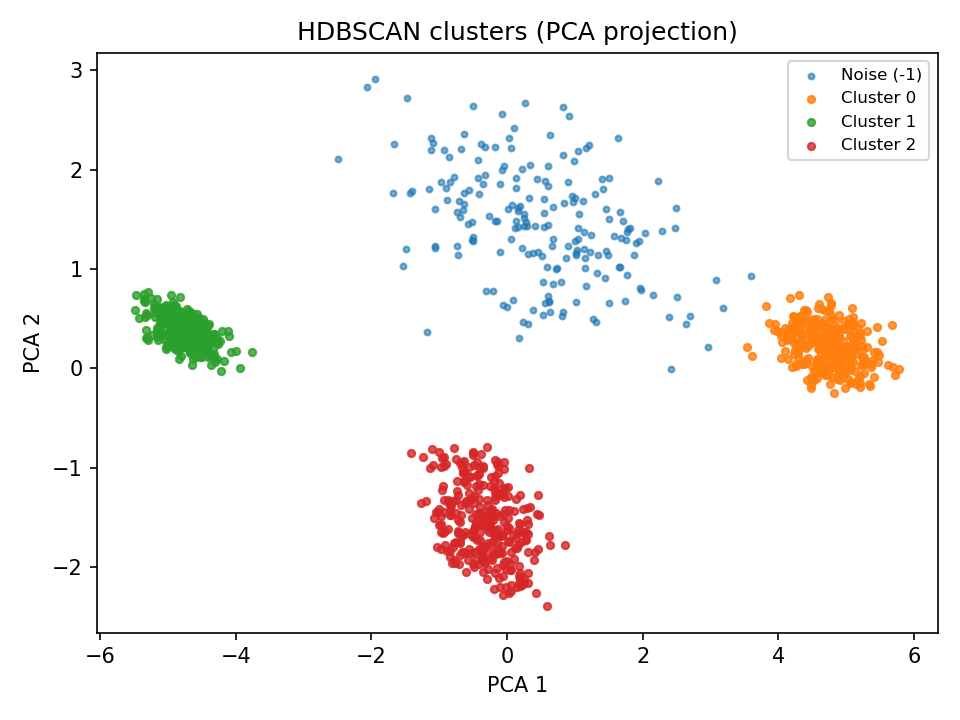
First, we can visualise how the clusters are separated. One way is to perform principal component analysis, and plot the clusters with x and y axes being the two principal components.

Next, we want to know which factors are separating the data into these different clusters. We can do by using the standard deviation values recorded in our results, do a little normalisation (since factors with bigger scores will naturally have bigger variations). Using the following code

import pandas as pd

df = pd.read_csv("student-stress-monitoring-datasets/versions/1/StressLevelDataset_hdbscan_clusters.csv")

# How many clusters, how big each is
print(df['cluster'].value_counts().sort_index())

# Summary stats by cluster
summary = df.groupby("cluster").mean(numeric_only=True)
# maximum value of each feature across entire dataset
max_vals = df.max(numeric_only=True)

# standard deviation of cluster means (between-cluster variance)
raw_var = summary.std()

# normalise by maximum value
normalized_var = (raw_var / max_vals).sort_values(ascending=False)

print("=== Normalised between-cluster variance ===")
print(normalized_var.round(4))

we get something like this

• mental_health_history — 0.4097
• stress_level — 0.4083
• social_support — 0.3919
• blood_pressure — 0.3191
• future_career_concerns — 0.2870
• sleep_quality — 0.2861
• bullying — 0.2846
• self_esteem — 0.2759
• anxiety_level — 0.2701
• teacher_student_relationship — 0.2636
• depression — 0.2629
• peer_pressure — 0.2548
• safety — 0.2537
• basic_needs — 0.2530
• academic_performance — 0.2525
• extracurricular_activities — 0.2491
• headache — 0.2412
• noise_level — 0.2106
• breathing_problem — 0.2054
• study_load — 0.2034
• living_conditions — 0.1630

This tells which factors contributes the most to the separation of the clusters. Next, let’s take a look at the histograms of the top 4 factors, mental_health_history, stress_level, social_support and blood_pressure. I will not be plotting the data points from cluster -1.

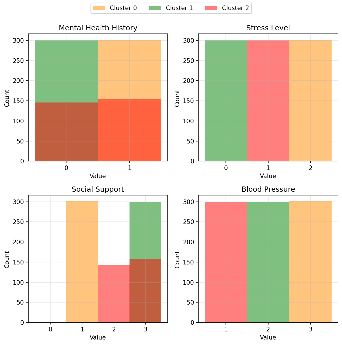
From these plots, we can start to interpret these clusters under broad categories:

• Cluster 0 - Highly stressed students with high blood pressure. They also have a history with mental health.
• Cluster 1 - Students that are generally doing well.
• Cluster 2 - Mildly stressed students but has low blood pressure.

These findings make sense. We expect, from experience, that stressed students exhibit a range of symptoms, like lack of sleep.

Conclusion

We find that stress levels are correlated with several other factors, including blood pressure, sleep quality, history of mental health .etc.

The question is are these factors causing each other? The data doesn’t tell us that. It will take more studies and more analysis to prove a direct causation between two factors.