I have used Gaussian process and it being used extensively in fields such as astrophysics. They are very useful and flexible models that can be applied to timeseries data. However, I often find it difficult to explain a Gaussian process (GP) to a non-expert in a short amount of time. While it is easy to use many of the GP libaries available, wrapping your head around the theoretical concepts can be challenging.

In this blog post, I will give an introduction to Gaussian processes to a non-expert who are interested in learning and using this stastical tool.

Motivation: A linear model

Let’s say that we have some data and we wish to fit out model to the data to infer its properties. We need a model that has the necessary flexibility to fit whatever shape our data is. If the data is simple enough, such as straight line with some noise, we can start with a simple linear model. We will define the model as \(\begin{align} f(x) = w_1 x + w_0. \end{align}\)

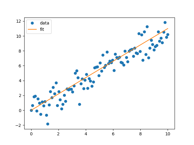
We will use this model to fit a straight line. We assume that our data is distributed along some Gaussian distribution, where \(\begin{align} y_i = \mathcal{N}(f(x), \sigma^2) \end{align}\) and hence we can think of our system as \(\begin{align} f(x) = w_1 x + w_0 + \epsilon. \end{align}\) where \(\epsilon\) is our noise term distributed accordingly to \(\mathcal{N}(0, \sigma^2)\). Now that we have defined our system, let’s fit a straight line to some data. To keep things simple, we will use optmisation instead of stochastic sampler as we care about only obtaining the best fit to prove my point. Since we assume the data is distributed along some Gaussian distribution, we define the Gaussian likelihood

and we use scipy.optimise.minimize to find the maximal likelihood and obtain the best fit

from scipy.optimize import minimize
import numpy as np
import matplotlib.pyplot as plt

sigma = 1

def neg_likelihood(alpha, y, x):
    f = alpha[1]*x + alpha[0]
    result = -np.prod((1/(2*np.pi*sigma))*np.exp(-(y-f)**2/(2*sigma)))
    print(result)
    return result

# make some data 

x = np.linspace(0, 10, 100)
y = x + np.random.normal(loc=0, scale=1, size=100)

# fit the data
result = minimize(
    neg_likelihood,
    x0 = np.array([0., 1.1]),
    args = (y, x),
)
params = result.x
y_fit = params[1]*x + params[0]

plt.figure()
plt.plot(x, y, linestyle='None', marker='o', label='data')
plt.plot(x, y_fit, label='fit')
plt.legend()
plt.show()

This is the data and the straight line fit. It looks pretty good. However, reality is never this simple and most of the time we don’t get data that can be fit by a straight line. What do we do, we can start increase the complexity and make the model more flexible.

Turn it up a notch: a quadratic model

We will use a more complex model with a quadratic model \(\begin{align} f(x) = w_2 x^2 + w_1 x + w_0 + \epsilon. \end{align}\) We will make the same assumption as before that the data is distributed as a Gaussian distribution. Performing the same operation as above, maximising the likelihood with our new model \(f(x)\). We get the following fit.

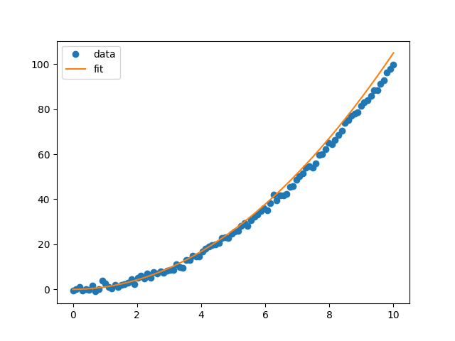
Okay, so as the features in the data becomes more complex, we need more complex models to fit the data. This is the aim of the game, to make a very flexible model to fit all of these really complicated features in the data that reality may throw at us. A simple way is to keep adding more and more to your model. We have already done this so far by considering the \(n=1\) and \(n=2\) case for the polynomial case and then we add \(x^3\) and \(x^4\) and so on.

Weight-space Formulation

We can start to get to what a Gaussian process is. We will begin our approach by creating a very flexible model by generalising the process of adding more features that we did in the previous section.

In our new model \(\mu\), we assume that there are a number of systematic effects that are not explicitly described by functions, but we know exists in the data. In other words, we don’t know weight of each of those systematics. Hence, we assign an unknown weight \(w\) for our systematics in our model

where \(\vec{w}\) is a vector containing the weight parameters, \(\begin{align} \vec{w}= \begin{bmatrix} w_0 \\ w_1 \\ \vdots\\ \end{bmatrix} \end{align}\)

and \(A\) is called a design matrix.

This design matrix represents how the weights affect our model \(f(\vec{w})\). You can think of this as the \(x\) and \(x^2\) terms of our model, except it is generalised to include terms \(x^p\) where p approaches very large. We are left with a massive matrix which allows much greater flexibility to model complicated datasets. We can define a standard likelihood for our data $y=[y_1, y_2, …, y_n]$ with Gaussian noise

Next, we put a zero mean Gaussian prior with convariance matrix \(\Lambda\) on the weights

and hence the prior can be written as

According the Bayes’ theorem, we can write the posterior as

Using the “magic of Gaussians” (the product of two Gaussian is a Gaussian), we can combine the two normal distributions to obtain \(\begin{align} p(\vec{w}|y, A) \propto \exp\left(-\frac{1}{2}|\vec{w}-\hat{\vec{w}}|^T \left(\frac{1}{\sigma^2}AA^T+\Sigma^{-1}\right)|\vec{w}-\hat{\vec{w}}|\right) \end{align}\)

where

\(\begin{align}\hat{\vec{w}}=\sigma^{-2}(\sigma^{-2}A^TA+\Sigma^{-1})A^Ty\end{align}\) \(\begin{align}=\sigma^{-2}\Lambda A^Ty \end{align}\).

where \(\begin{align} \Lambda = \sigma^{-2}A^T A+ \Sigma^{-1} \end{align}\)

this \(\hat{\vec{w}}\) is the mean of our Gaussian process result. We now have someting that looks like a Gaussian distribution, aka. \((y-mean)^Tcov^{-1}(y-mean)\). We have our mean and now we want our covariance matrix. Now, let’s project to some input data, which I will refer to as \(\phi(x_*)\) which creates some output \(y\)

Using the Woodbury matrix identity

To make predictions using this equation, we need to invert the \(\Lambda\) matrix. As we project the data to higher and higher dimensions, we need to construct an ever bigger design matrix, which becomes computationally intractable as we increase the number of dimension. However, due Mercer’s theorem, where any inner product of matrices can be replaced by a function as long as it returns a positive semi-definite matrix. This function is the kernel function

This is very convenient as we can recast our problem in terms of the kernel function instead of computing the inner product of infinite dimensional matrices. What this means is that you can represent relations in higher dimensions by using correlations between the data points in the lower dimension coordinates (between \(x\) and \(x'\)), instead of transforming and representing the data in the higher dimensional feature space. This is called the kernel trick and it is incredibly useful.

Thus,

We can marginalise out \(\hat{\vec{w}}\)

where \(p(y_*\vert x_*,\hat{\vec{w}})\) is our likelihood for a single data point,

and I will skip a lot of math and state the final result below

if we define \(k(x_*, x_*')=\phi^T\Sigma\phi\), it becomes

Function-space Formulation

The formal definition of a Gaussian process is a collection of random variables, any finite number of which have a joint Gaussian distribution. You can think of this as all the data is drawn from a huge multivariate Gaussian distribution. A Gaussian process is completely specified by the mean \(\mu(x)\) and the covariance \(\Sigma(x, x')\) and we can write the Gaussian process as

The covariance matrix describe how each data point is correlated with each other. As a result, you can generate an infinite number of functions that could describe the data.

A Gaussian processes assign a prior probability to each of the infinite number of possible functions. We are not interested in having an infinitely many possible functions. To constrain the number of possible functions we can draw from the GP, we can either

1. change the covariance matrix
2. incorporate our observational data

For the former, this bring us to our kernel function \(k(x, x')\) we defined in the previous section. Since the covariance can be written in terms of kernel functions, we can change the covariance matrix to constrain how the data points are correlated. You can think of this as if you are telling how the data should correlated, you are placing a prior assumption on what functions can model your data and reduce that infinite number of possible to function to a “slightly less infinite” number of functions that are btter at modelling your data.

Kernels

We have shown that the data in the higher dimensional space can be described by a kernel function, but what kernel functions can we use. Kernels can be classified into stationary or non-stationary. Stationary kernels depends the relative distance between data points, which you can think of modelling an effect independent of time. On the other hands, non-stationary kernels depend on the value of the input value, which models an effect at a specific, local point in time.

Each kernel function has its own parameters (we call them hyperparameters). They do not directly describe the data, but describe the structure within the covariance matrix, which then describes the data. Here are few different types of commonly-used kernels which can be used as is or in combination with other kernels.

Radial basis function (squared-exponential) kernel

This is a infinitely differentiable (aka. smooth), stationary kernel. It is parameterised by the length hyperparameter \(l\), which defines the length scale of data correlated with each other. A high \(l\) results in more further data points being correlated and the function appears more structured. A low \(l\) results in less data points being correlated and the function appears more chaotic.

Matern kernel

This is generalisation of the radial basis function kernel. It is also stationary. The hyperparameter \(\nu\) controls the smoothness of the function, with \(\nu \rightarrow \infty\) case being equivalent to the radial basis function kernel. \(\nu=3/2\) is once differentiable and \(\nu=5/2\) is twice differentiable. The kernel can be useful if you don’t want your functions to be smooth. You can have a situation where you data appears discontinuous, and the need of a non-smooth function.

These are draws from a matern-3/2 kernel. Notice how it is much more jagged then the radial basis function kernel.

Exp-Sine-Squared (periodic) kernel

As the name suggests, this kernel allows functions to be periodic. This hyperparameter \(p\) controls the periodicity and the length hyperparameter \(l\) controls the length scale.

These are draws from a periodic kernel.

There are many more kernels out there!

Code packages and examples

There are a wide variety of Gaussian process python libaries with different implementations. The greatest challenge to computing a GP comes from inverting the covariance matrix \(C+A\Lambda A^T\), which has the computational complexity of \(\mathcal{O}(n^3)\). Hence, the aim of the game is to reduce the complexity down. Some implementations is able to do this by using certain mathematical property’s under special conditions.

Here is the list of the code packages

• George: python libary that implements GPs. You can use both stationary and non-stationary kernels. It primarily use two solvers, which are scipy’s Cholesky implementation and Sivaram Amambikasaran’s HOLDLR algorithm.
• celerite: uses sums of complex-valued exponent as the kernel. This special kernel allows the computational cost of the GP to scale linearly with number of data points.
• tinygp: built on top of JAX, which allows for GPU acceleration and automatic differentiation.

Celerite example and predictions in missing data

Here is an example taken from the celerite example with simulated data (click the link for more details). We have data except for a region between 3.8 s and 5.5 s. Now, we do the two things we mention before, choose a kernel function and condition our GP to our observational data. Since the simulated data looks periodic and is linearly increasing, we will need a function that allows our data is periodic and extra flexibility to make it increase. hence, we choose the double simple harmonic oscillator. Next, we condition our GP to the observational data. To condition to our data, we must solve the inverse data problem, figure out what hyperparameters will lead to the GP to fit our data. This can be done by using an optimiser or a stochastic sampler. For this example, we will use a optimiser as they tend to be quicker. I have provided the code below.

import numpy as np
import matplotlib.pyplot as plt
from celerite import terms
from scipy.optimize import minimize

np.random.seed(42)

t = np.sort(np.append(
    np.random.uniform(0, 3.8, 57),
    np.random.uniform(5.5, 10, 68),
))

yerr = np.random.uniform(0.08, 0.22, len(t))
y = 0.2 * (t-5) + np.sin(3*t + 0.1*(t-5)**2) + yerr * np.random.randn(len(t))

true_t = np.linspace(0, 10, 5000)
true_y = 0.2 * (true_t-5) + np.sin(3*true_t + 0.1*(true_t-5)**2)

# A non-periodic component
Q = 1.0 / np.sqrt(2.0)
w0 = 3.0
S0 = np.var(y) / (w0 * Q)
bounds = dict(log_S0=(-15, 15), log_Q=(-15, 15), log_omega0=(-15, 15))
kernel = terms.SHOTerm(log_S0=np.log(S0), log_Q=np.log(Q), log_omega0=np.log(w0),
                       bounds=bounds)
kernel.freeze_parameter("log_Q")  # We don't want to fit for "Q" in this term

# A periodic component
Q = 1.0
w0 = 3.0
S0 = np.var(y) / (w0 * Q)
kernel += terms.SHOTerm(log_S0=np.log(S0), log_Q=np.log(Q), log_omega0=np.log(w0),
                        bounds=bounds)

gp = celerite.GP(kernel, mean=np.mean(y))
gp.compute(t, yerr)  # You always need to call compute once.

def neg_log_like(params, y, gp):
    gp.set_parameter_vector(params)
    return -gp.log_likelihood(y)

initial_params = gp.get_parameter_vector()
bounds = gp.get_parameter_bounds()

r = minimize(neg_log_like, initial_params, method="L-BFGS-B", bounds=bounds, args=(y, gp))
gp.set_parameter_vector(r.x)

x = np.linspace(0, 10, 5000)
pred_mean, pred_var = gp.predict(y, x, return_var=True)
pred_std = np.sqrt(pred_var)

color = "#ff7f0e"
plt.errorbar(t, y, yerr=yerr, fmt=".k", capsize=0, label='data')
plt.plot(x, pred_mean, color=color, label='mean')
plt.fill_between(x, pred_mean+pred_std, pred_mean-pred_std, color=color, alpha=0.3,
                 edgecolor="none", label=r'$1-\sigma$ interval')
plt.xlabel("x")
plt.ylabel("y")
plt.xlim(2, 8)
plt.ylim(-2.5, 2.5)
plt.legend()
plt.savefig('GP_example.png')

Just like the visual example above, we make many draws from the GP (the multivariarte Gaussian distribution) to see what the model prediction looks like. To make sense of many draws, we usually plot the mean (or median) of these draws and the \(1\sigma\) interval. This shows what the average looking draw looks like, and the \(1\sigma\) interval acts as an error bar. As we can see in the plot below, the GP is conditioned and fits the data and we see that for the missing data points, there is a prediction with some uncertainty made by the GP.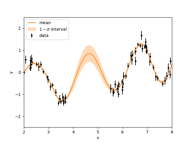

Conclusion

We show that by taking a linear model in the data space, we can make it more flexible by imbedding it in a higher dimensional feature space. Additionally by applying the kernel trick, we are able to describe the correlations between the data using a kernel function instead of taking a inner product. As a result, we have a very flexible model where the data is described by a multivariate Gaussian distribution, which is described by a covariance matrix.

I hope this introduction has been helpful. There are several ready-to-use python GP libraries and hence I recommend people to use them if they find GPs are applicable to the problem. Choosing the appropriate kernel function can be unclear, and it depends on what you believe the signal you are fitting should look like.

References

• Gaussian Processes for Machine Learning, Carl Edward Rasmussen and Christopher K. I. Williams The MIT Press, 2006. ISBN 0-262-18253-X.
• A Practical Guide to Gaussian Processes
• The Kernel Trick in Support Vector Classification
• gaussian-process-not-quite-for-dummies
• Fast and scalable Gaussian process modeling with applications to astronomical time series, arXiv:1703.09710, Foreman-Mackey et al..