In the field of Gravitational-Wave astronomy, I see a transition from traditional stochastic sampling methods such as Monte Carlo Markov Chains and nested sampling towards something called normalising flows. As our inference problems become harder due to the increasing volume of data, we need faster inference methods. In this blog post, we will go through what is a normalising flow and can it solve inference problem that are intractably long for traditional methods.

Theoretical background

A normalising flows works by transforming a simple probabilty distribution (usually a Gaussian distribution) into a more complex distribution through a sequence of mappings. Let \(X\) be a random variable with a tractable probability density function \(p_X\). We want to transform this distribution \(p_X\) (source distribution) into distribution \(p_Y\) (target distribution) using an invertible (bijective) function \(g\) where

We can also transform \(p_Y\) back into \(p_X\) using the inverse function \(g^{-1}\).

Change of variables

If we want to figure out the probability value close to a particular Y value, we look at the area under a small interval \(dx\). We can do something similar for X.

substituting \(x\) with the inverse function \(g^{-1}(y)=x\), we have the formula

where the term \(\vert \frac{\partial g(g^{-1}(y))}{\partial x}\vert\) is the Jacobian. One job for the Jacobian is to ensure the new probability density normalises to 1. The new probability density function \(p_Y(y)\) is called a pushforward of the density \(p_X\).

The function \(g\) (the generator) pushes forward the original density \(p_X\) to a more complex density. This movement where the simple density flows to a more complex density it called the generative direction. We can take the inverse function \(g^{-1}\) and use it to move in the opposite direction, turning from a complex distribution into a more simple distribution. Hence, this is why it is named normalising flows, we applying invertible transformations to transform probability distributions while ensuring they are normalised.

Generative model likelihood

An obvious use for normalising flows is to perform parameter estimation. We assume that there is a only a single flow parameterised by \(\theta\) and the original distribution is parameterised by \(\phi\). We need to derive a likelihood function to evaluate the data with given parameters \(\psi = (\theta. \phi)\). We can simply take the previous equation and take the logarithm on both sides, which results in our log likelihood function

where the first term is the log likelihood under the original distribution and the second term accounts for the change of volume induced by the transformation of the normalising flows.

Implementing normalising flows

Normalising flows should satisfy the following conditions in order to be practical:

• be invertible.
• be sufficiently expressive to model the distribution of interest.
• be computationally efficient, at computing \(g\), \(g^{-1}\) and also the determinant of the Jacobian.

Constructing a complicated bijective function can be difficult. One approach is to use a simpler bijective function to compose a much more complicated function. A composite function \(g\) made of \(N\) invertible function \(\{g_i\}_{i=0}^{N}\) is itself invertible and the determinant of its Jacobian has a specific form. Hence, \(g\) is bijective and the inverse

and the determinant of the Jacobian is

Thus, we can use multiple bijective functions to compose a more complicated function.

Coupling flows

A trick for reducing the computational cost of a flow is to ensure that the Jacobian is triangular (where the \(i>j\) or \(i<j\) elements in a matrix is zero). Since we wish to calculate the determinant of the Jacobian in our likelihood function, only the diagonal of the matrix will give a non-zero value as the upper (or lower) triangular of the matrix has zero values, hence the off-diagonal terms in the determinant calculation is zero.

One way to ensure the Jacobian is triangular is by using a coupling layer. Consider the input \(x \in \mathcal{R}\) into two subspaces \(x_A\) and \(x_B\) and a bijective function \(h\). For the first subset, we use two functions, \(h\) and \(\Theta\), where \(\Theta\) is an input to \(h\):

and we also need \(h\) to be invertible so that

The graph below visually demonstrates how the coupling layer works .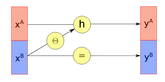

In this particular transformation, the Jacobian will be upper tringular:

as \(y_B = x_B\) implies that lower right element is 1 and as the second subset is completely independent of the first subset, the lower left element is 0.

Affine coupling

Now that we introduce coupling flows, a question that natually arises is what should the coupling function \(h\) be? One architectures called nonlinear independent component (NICE) proposed by Dinh et al. (2015) has a simple additive function:

where \(T\) is known as a translation function. Another architecture called real non-volume preserving (R-NVP) flow proposed by Dinh et al. (2017) uses an affine coupling function:

where \(T\) is the same translation function as before and \(S\) is a scaling function. The functions are both simple and easier to compute. However, the drawback is that you need to stack many functions together to represent complicated distributions.

Code example

Gaussian to two moons

Let’s go through an example where we fit a complex 2D distribution using a normalising flow. We will use a normalising flow to fit the two moons dataset in sklearn.dataset. The reason why I chose this type of dataset is because it is a fairly complicated distribution, it is non-Gaussian, non-linear and multi-modal, which is not something that a linear transformation or a single affine function can fit. We will use the R-NVP architecture and the affine coupling function. Through the example, I want to show you that using a composition of simple affine functions, we can use a normalising flow to fit something fairly complicated.

I wil use python code and use PyTorch code package library, which has a neural network subpackage. We construct the neural network using the torch.nn.linear which applies a affine linear transformation to the data and a rectified linear unit (ReLU) layer in between the linear layers.

The neural network is now Linear -> ReLU -> Linear -> ReLU -> Linear.

I have included the code below.

import numpy as np
import torch
import torch.nn as nn
from sklearn.datasets import make_moons
import matplotlib.pyplot as plt


def sample_two_moons(n=100, noise=0.1, device="cpu"):
    x, _ = make_moons(n_samples=n, noise=noise)
    x = torch.tensor(x, dtype=torch.float32, device=device)
    return x


class MLP(nn.Module):
    def __init__(self, in_dim, out_dim, hidden=128):
        super().__init__()
        self.net = nn.Sequential(
            nn.Linear(in_dim, hidden),
            nn.ReLU(),
            nn.Linear(hidden, hidden),
            nn.ReLU(),
            nn.Linear(hidden, out_dim),
        )
        
    def forward(self, x):
        return self.net(x)


class AffineCoupling(nn.Module):

    def __init__(self, dim=2, mask=None, hidden=128, scale_clip=2.5):
        super().__init__()
        assert dim == 2
        if mask is None:
            mask = torch.tensor([1.0, 0.0])
        self.register_buffer('mask', mask.view(1, dim))
        self.s_net = MLP(dim, dim, hidden)
        self.t_net = MLP(dim, dim, hidden)
        self.scale_clip = scale_clip

    def forward(self, x):
        x_masked = x * self.mask
        s = self.s_net(x_masked) * (1 - self.mask)
        t = self.t_net(x_masked) * (1 - self.mask)
        
        s = torch.tanh(s) * self.scale_clip
        
        y = x_masked + (1 - self.mask) * (x * torch.exp(s) + t)
        
        log_det = s.sum(dim=1)
        return y, log_det
    
    def inverse(self, y):
        y_masked = y * self.mask
        s = self.s_net(y_masked) * (1 - self.mask)
        t = self.t_net(y_masked) * (1 - self.mask)
        s = torch.tanh(s) * self.scale_clip
        
        x = y_masked + (1 - self.mask) * ((y-t) * torch.exp(-s))
        log_det_inv = (-s).sum(dim=1)
        return x, log_det_inv
    
class Flow(nn.Module):
    def __init__(self, layers): 
        super().__init__()
        self.layers = nn.ModuleList(layers)
    
    def forward(self, x):
        log_det_sum = torch.zeros(x.shape[0], device=x.device)
        z = x
        for layer in self.layers:
            z, log_det = layer.forward(z)
            log_det_sum += log_det
        return z, log_det_sum
    
    def inverse(self, z):
        log_det_sum = torch.zeros(z.shape[0], device=z.device)
        x = z
        for layer in reversed(self.layers):
            x, log_det = layer.inverse(x)
            log_det_sum += log_det
        return x, log_det_sum
    
    
    
def normal_log_prob(z):
    return -0.5 * (z**2).sum(dim=1) - z.shape[1] * 0.5 * np.log(2 * np.pi)


device = "cuda" if torch.cuda.is_available() else "cpu"

masks = [torch.tensor([1.0, 0.0]),
         torch.tensor([0.0, 1.0])]

layers = []

n_layers = 8

for i in range(n_layers):
    layers.append(AffineCoupling(dim=2, mask=masks[i % 2], hidden=128, scale_clip=2.5))

flow = Flow(layers).to(device)
opt = torch.optim.Adam(flow.parameters(), lr=2e-3)

batch_size = 1024
steps = 4000

for step in range(1, steps + 1):
    x = sample_two_moons(batch_size, noise = 0.06, device=device)
    
    z, log_det = flow.forward(x)
    log_pz = normal_log_prob(z)
    log_px = log_pz + log_det
    
    loss = -log_px.mean()
    
    opt.zero_grad()
    loss.backward()
    opt.step()
    
    if step % 500 == 0 or step == 1:
        print(f"step {step:4d} | NLL {loss.item():.3f}")

with torch.no_grad():
    z = torch.randn(5000, 2, device=device)
    x_samp, _ = flow.inverse(z)

    x_data = sample_two_moons(5000, noise=0.06, device=device)

# Convert back to numpy
x_samp = x_samp.cpu().numpy()
x_data = x_data.cpu().numpy()

# Plot the original samples

fig, ax = plt.subplots(figsize=(8, 4))
ax.scatter(x_data[:, 0], x_data[:, 1], s=5, alpha=0.4, label="Target (two moons)")
ax.scatter(z[:, 0], z[:, 1], s=5, alpha=0.4, label="Flow samples")
ax.set_aspect("equal", "box")
ax.legend()
ax.set_title("Original samples from Gaussian")
plt.tight_layout()
plt.savefig('two_moons_plot_before.png')
plt.show()

# Plot the samples after training normalising flow
fig, ax = plt.subplots(figsize=(8, 4))
ax.scatter(x_data[:, 0], x_data[:, 1], s=5, alpha=0.4, label="Target (two moons)")
ax.scatter(x_samp[:, 0], x_samp[:, 1], s=5, alpha=0.4, label="Flow samples")
ax.set_aspect("equal", "box")
ax.legend()
ax.set_title("Normalising flow: Gaussian to two moons")
plt.tight_layout()
plt.savefig('two_moons_plot.png')
plt.show()

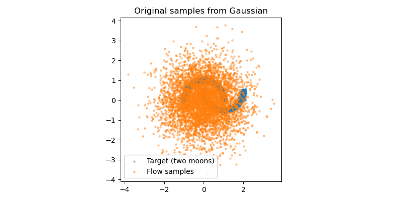
Let’s see how well we are able to fit the two moons distribution. First, I have plot the samples drawn from the 2D Gaussian distribution, which are our original samples.

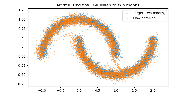
However, by using the normalising flow, we are able to transform the samples from a simple 2D Gaussian dsitribution into the more complex two moons distribution. You can think of the transformation as the collection samples in the original Gaussian distribution slowly compressing and warping into the two moons shape as we continuously train the normalising flow.

Conclusion

In this blog post, I have introduced the basics of a normalising flow. Using a composition of simple bijective functions, we can express a complicated distribution from a simple distribution. This is an immensely useful method, as it allows people to fit complicated datasets using simple functions rather than having to create a very complicated and cumbersome model. Furthermore, the time and computational cost to train and use a normalising flow can be much lower in total compared to other traditional methods of fitting complicated datasets such as Monte-Carlo Markov Chain or nested sampling. Hence, I can see normalising flow has potential for many applications in astrophysics and beyond.

References

• Normalizing Flows: An Introduction and Review of Current Methods, Ivan et al. (2019)
• Normalizing flows: Explicit distribution modeling, Ashish Jha, 12/10/2023
• What are normalising flows, Ari Seff, 7/12/2019
• Normalizing Flows, Grishma Prasad (2021).
• NICE: Non-linear Independent Components Estimation, Dinh et al. (2015)
• Density estimation using Real NVP, Dinh et al. (2017)